
PID is acronym for Proportional Plus Integral Plus Derivative Controller.It is a control loop feedback mechanism (controller) widely used in industrial control systems due to their robust performance in a wide range of operating conditions & simplicity.In This PID Controller Introduction, I have Tried To Illustrate The PID Controller With SIMPLE Explanations & BASIC MATLAB CODE To Give You Idea About P,PI,PD & PID Controllers
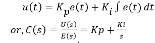
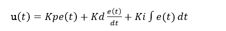
For PID control, the actuating signal u(t),consists of proportional error signal added with derivative and integral of error signal e(t)

The Plant P is controlled by input u(t) which is represented as

Where Kp is the Proportional Gain,Kd is the Derivative Gain & Ki is the Integral Gain of the controller
Frequency Domain Representation of PID Controller
In Frequency Domain (after taking Laplace Transform of both sides),the control input can be represented as

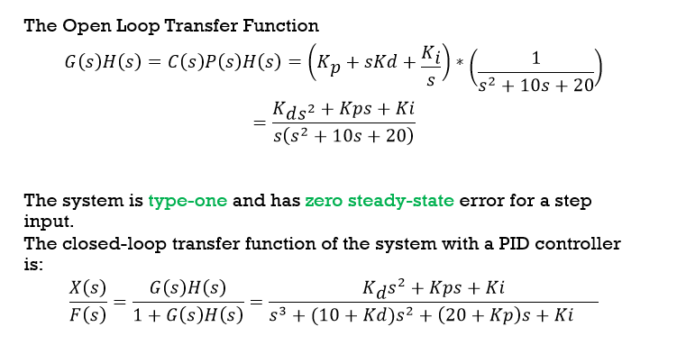
Thus ,PID controller adds pole at the origin and two zeroes to the Open loop transfer function
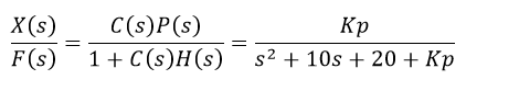
The Closed loop Transfer Function of the system can be written as
![]()
Physical Realisation of PID Controller

Why do You Need a PID Controller
The Characteristics of P, I, and D controllers are briefly discussed With MATLAB Code to give an insight about individual P,PI,PD,PID Controllers
- A proportional controller (Kp) will have the effect of reducing the rise time and will reduce, but never eliminate, the steady-state error.
- An integral control (Ki) will have the effect of eliminating the steady-state error, but it may make the transient response worse.
- A derivative control (Kd) will have the effect of increasing the stability of the system, reducing the overshoot, and improving the transient response but little effect on rise time
- A PD Controller could add damping to a system, but the steady-state response is not affected.(steady state error is not eliminated)
- A PI Controller could improve relative stability and eliminate steady state error at the same time, but the settling time is increased(System response sluggish)
But a PID controller removes steady-state error and decreases system settling times while maintaining a reasonable transient response
Example::Illustrating P, PI, PD & PID controller in MATLAB
For the Given Spring-Mass-Damper System
Using D’Alembert’s Principle


Taking Laplace Transform with Zero initial conditions to get:
![]()
The transfer function between Output X(s) & input F(s) is
![]()
Assuming m=1kg,b=10 Ns/m & k=20 N/m [For Simpicity]
![]()
Which is the open loop transfer function
On Matlab Command window, typing following commands, yield Step Response of the system
G=tf(1,[1 10 20]);
Step(G);

The DC gain of the plant transfer function is 1/20, so 0.05 is the final value of the output to a unit step input. This corresponds to the steady-state error of 0.95, quite large indeed.
Furthermore, the rise time is about one second, and the settling time is about 1.5 seconds.
#Proportional Control
In Proportional control, the actuating signal for the control action in a control system is proportional to the error signal. The error signal being the difference between the reference input signal and the feedback signal obtained from the output

The Transfer function of the controller is:
U(s) = Kp E(s) or, C(s) =Kp
The closed-loop transfer function of the Spring-Mass system with a proportional controller is:
For Kp=500
Executing following Commands in MATLAB will give output on command window
Kp = 500;

C = pid(Kp)

P=tf(1,[1 10 20])

T = feedback(C*P,1)

t = 0:0.01:2;

step (T,t);

The Step response of the system in MATLAB indicates that the proportional controller (Kp) reduces the rise time, increases the overshoot, reduces the steady state error but never eliminates it completely
This is a type-zero system and hence will have a finite steady-state error for a step input.

Large values of K lead to small steady-state error; however, they also lead to a faster, less damped responses.
If we want a small overshoot and a small steady-state error, a proportional gain alone is not enough.
#PD Controller
For Derivative control action the actuating signal consists of proportional error signal added with derivative of the error signal

A proportional plus derivative (PD) controller has the transfer function:

Proportional-derivative (PD) control considers both the magnitude of the system error and the derivative of this error. Derivative control has the effect of adding damping to a system, and, thus, has a stabilizing influence on the system response.
The closed-loop transfer function of

the above system with a PD controller is:
—
MATLAB Code for PD Controller(Without Tuning Sample Values)
Entering Following commands in MATLAB yields
| Kp = 500;
Kd=10; C = pid(Kp,0,Kd); P=tf(1,[1 10 20]); T = feedback(C*P,1) step(T); |
Continuous-time PD controller in parallel form:
Kp + Kd * s
With Kp = 500, Kd = 10
Transfer function:
10 s + 500
—————-
s^2 + 20 s + 520
Without integral control, this is a type-zero system, and hence will have a finite steady state error to a unit step input

The derivative controller reduced both the overshoot and the Settling time, and had a small effect on the rise time and the steady-state error.
The PD controller has decreased the system settling time considerably; however, to control the steady-state error, the derivative gain Kd must be high. This decreases the response times of the system and can make it susceptible to noise.
Effects of PD Controller :-
- Improves damping and maximum overshoot.
- Reduces rise time & settling time.
- Increases Bandwidth
- Improves Gain Margin and Phase Margin
- May attenuate high frequency noise
#PI Controller
For Integral control action, the actuating signal consists of proportional-error signal added with integral of the error signal.
Proportional-integral (PI) control considers both the magnitude of the system error signal and the integral of this error

MATLAB Code for PI Controller(Without Tuning Sample Values)
Executing Following commands in MATLAB
Kp = 30;

Ki=70;

C = pid(Kp,Ki)

P=tf(1,[1 10 20]);

T = feedback(C*P,1)

step(T);
| Continuous-time PI controller in parallel form:
1 Kp + Ki * — s With Kp = 30, Ki = 70 Transfer function: 30 s + 70 ———————— s^3 + 10 s^2 + 50 s + 70 |

Using integral control makes the system type-one, so the steady-state error due to a step input is zero.
The response shows that the Integral control has removed the steady-state error and improved the transient response, but it has also increased the system settling time.

Increasing Ki increases overshoot & settling time making system response sluggish
To reduce both settling time and overshoot, a PI controller by itself is not enough
Effects of PI Controller :-
- Improves damping and reduces maximum overshoot.
- Increases Rise Time.
- Decreases Bandwidth
- Improves Gain Margin, Phase margin & Peak Resonance (Mr).
- Filter out high frequency noise.
PID Controller
For PID control, the actuating signal u(t),consists of proportional error signal added with derivative and integral of error signal e(t)
Proportional-integral-derivative control (PID) combines the stabilizing influence of the derivative term and the reduction in steady-state error from the integral term.
The Transfer function of PID Controller


MATLAB Code for PID Controller(Without Tuning Sample Values)
MATLAB Code to Be Executed for Simulating PID Controller
Kp=500,Kd=50,Ki=400;

G=tf(1,[1 10 20]);

C=pid(Kp,Ki,Kd);

T=feedback(C*G,1);

step(T,0:0.01:2);
| MATLAB OUTPUT FOR Continuous-time PID controller in parallel form:
1 Kp + Ki * — + Kd * s s With Kp = 500, Ki = 400, Kd = 50 Transfer function: 50 s^2 + 500 s + 400 ————————– s^3 + 60 s^2 + 520 s + 400 |

Thus, A PID controller has removed steady-state error and decreased system settling times while maintaining a reasonable transient response
While designing a PID controller, the general rule is to add proportional control to get the desired rise time, add derivative control to get the desired overshoot, and then add integral control (if needed) to eliminate the steady-state error.
Effects of PID Controller:-
- Its purpose is to improve stability as well as to decrease Steady State Error.
- It adds a pole at origin which increases type of system which result into reduction of steady state error.
- It adds 2 zeroes in LHP, one finite zero to avoid effect on stability & other zero to improve stability of system
Applications of PID Controller
- Proportional-Integral-Derivative (PID) control is the most common control algorithm used in industry and has been universally accepted in industrial control. This is due to the fact that all design specifications of the system can be met through optimal tuning of constants Kp, Ki & Kd for maximum performance
- In the early history of automatic process control the PID controller was implemented as a mechanical device in steering system of Ships
- PID temperature controllers are applied in industrial ovens, plastics injection machinery, hot stamping machines and packing industry.
- Electronic analog PID control loops are often found within more complex electronic systems, for example, the head positioning of a disk drive, the power conditioning of a power supply, or even the movement-detection circuit of a modern seismometer.
- Most modern PID controllers in industry are implemented in programmable logic controllers (PLCs) or as a panel-mounted digital controller.
Limitations of PID Controllers
- The performance of PID controllers in non-linear systems (such as HVAC systems) is variable because PID controllers are linear
- The derivative term Kd is susceptible to Noise disturbance. A small amount of measurement or process noise can cause large amounts of change in the output. It is often helpful to filter the measurements with a low-pass filter in order to remove higher-frequency noise components
- The PID Parameters need to be tuned in order to obtain required optimal response
- Doesn’t handle non‐symmetric systems very well (e.g. A system which heats much faster than it cools)